0. 概要 Outline
本文提供了一种用卷积神经网络(CNN)估计离散选择模型的方法,从而使神经网络强大的预测能力可以在选择预测问题上得以发挥。通过实验发现:一个单层+单卷积核+无激活函数的CNN与MNL模型是完全等价的;多层+多卷积核+非线性激活函数的CNN可以非常好地解决MNL中不可避免的效用非线性的问题;然而,这样的CNN在处理复杂的模型形式(如NL)时却无能为力。这意味着,当MNL模型需要优化时,常见的两个方向——解释变量精细化和模型形式精细化中,前者可用CNN解决,后者只能留给精细化模型自己。
This article presents a method of estimating discrete choice models using convolutional neural network (CNN), so that the powerful predicting abilities of neural network could be utilized in choice situations. Three results are shown through experiments: 1) a MNL model is completely equivalent to a CNN with 1 convolutional layer, in which there only 1 out channel and no nonlinear activation; 2) CNN with multiple convolutional layers + multiple out channels in each layer + nonlinear activation could greatly solve the nonlinear utility problem which is nearly inevitable in practice; 3)however, such CNN could not solve the problems concerning the more complex discrete choice models, such as nested logit model.
When a MNL model needs to be improved, there are generally 2 main directions. The one is to better specify the utilities, such as introducing nonlinear terms; the other is to replace the MNL form using more refined NL, MXL, etc. From the findings above, the former could be achieved by CNN, while the latter not.
下面的实验通过”PythonCode.zip”中3段Python代码实现:”identical_simple_cnn_mnl.py”展示了CNN与MNL的等效性;”complex_cnn.py”展示了CNN在处理非线性效用时的强大能力;”nested_logit.py”反映了CNN无法处理由精细化模型带来的复杂性。
There experiments are conducted using 3 pieces of Python codes in ‘PythonCode.zip’. ‘identical_simple_cnn_mnl.py’ shows a simple CNN could be equivalent to MNL; ‘complex_cnn.py’ shows how CNN well performs when utilities in MNL are nonlinear; ‘nested_logit.py’ shows CNN is incapable of more complex models, such as nested logit model.
1. 用CNN实现MNL (Generating the Same Results of MNL Using CNN)
神经网络在许多预测性问题上的表现有目共睹,然而却很少应用在关于“个体选择”的预测上。另一方面,离散选择模型作为处理选择问题的传统方法,也常常受到线性效用设定的约束,需要神经网络强大的非线性能力。
Neural network has outstanding reputation in many kinds of prediction problems, however, it is seldom used in predicting individual choices. At the same time, discrete choice models generally assume linear utilities, which are problematic in many occasions and thus need the powerful nonlinearity of neural network.
有人可能会想:神经网络常用的分类问题与选择问题有相似之处,因变量都是离散的,能否直接推广?答案可能没那么简单,因为二者的数据形式是不同的。分类问题中,1个样本的1个解释变量通常只有1个值,例如:根据体温判断“有病/没病”,每个就诊者的体温是1个数值。而在N个备选项的选择问题中,1个样本的1个解释变量常常有N个值 ——每个备选项1个,例如,出行者根据行程时间选择“公交/出租车/步行”3种交通方式时,每1种交通方式都对应1个行程时间,共3个行程时间。由于这种差别,分类问题通常是1行数据对应1个样本;而选择问题常常采用长表形式,每N行组成一个“组”,共同对应1个样本,下表是交通方式选择的2个样本。其中,Group代表样本编号,Alt代表备选项名称,Choice是选择结果,每一组中有且只能有一个“1”,代表该行的备选项被选中,其他的“0”代表未被选中。
People may believe that we could generalize the applications of neural network in classification to choice, since the dependent variables are discrete in both classification and choice. However, it might not that easy, because the data format are different in classification and choice problems. For any explanatory variable, one case usually has ONLY ONE value in a classification problem; by contrast, in a choice problem with N alternatives, one case usually has N dependent values for certain explanatory variable, that is to say, each alternative would have a corresponding value. For example, when travelers choose traffic modes among bus/ taxi /walk according travel time, each mode has its own travel time. Consequently, it is general to have only one row for a case in a classification problem, while in a N-alternative choice problem, a case often need N rows to be a group, as shown in the following table, 2 cases corresponds to 6 rows.
| Group | Alt=alternative | Choice | TT = travel time (min) | Price (¥) |
| 1 | Bus | 1 | 20 | 2 |
| 1 | Taxi | 0 | 10 | 20 |
| 1 | Walk | 0 | 70 | 0 |
| 2 | Bus | 0 | 40 | 5 |
| 2 | Taxo | 0 | 10 | 20 |
| 2 | Walk | 1 | 100 | 0 |
怎样用神经网络处理这样的数据呢?如果采用传统的全连接形式,对于“行程时间”和“价格”两个变量,由于有3个备选项,就要使用6个输入节点,分别代表“公交行程时间”、“出租车行程时间”、“步行行程时间”、“公交价格”、“出租车价格”、“步行价格”,这样虽然也是可行的,但是感觉上怪怪的。尽管神经网络并不强调解释性,但隐藏层节点同时连接所有选项的所有属性,又有什么实际意义呢?
How to deal with this kind of data using neural network? If we adopt classical fully connected neural network, 6 inputs nodes are needed to handle the 2 variables (TT and Price), which stand for ‘Bus TT’, ‘Taxi TT’, ‘Walk TT’, ‘Bus Price’, ‘Taxi Price’, ‘Walk Price’ respectively. This way should also work, but seems a little bit strange.
因此,换一种形式吧。我们都知道,根据神经网络的设定,如果没有隐藏层,且最后不用非线性的激励函数的话,一个神经网络就完全等价于一个线性回归。那么,有没有一种神经网络的形式,能完美地等价于离散选择模型中最经典的多项Logit(MNL)模型呢?
As we all know, a fully connected neural network without hidden layers and nonlinear activation functions would just equal to a linear regression. Similarly, I wonder if there is a certain kind of neural network completely equal to MNL.
看一看MNL中的设定吧。上例中,我们可以采用两个参数——b(TT)和b(Price)建立MNL模型,V代表每个备选项的可见效用,P代表选择概率。注意到,对于不同的选项,行程时间与价格的系数是相同的;同时,为了简单考虑,这里没有使用常数项。
Let’s revisit the specification of MNL. In the case above, we could use two coefficients, b(TT) and b(Price) to specify a MNL model, as shown below. Constants are omitted for simplicity.
V(Bus) = b(TT) * TT(Bus) + b(Price) * Price(Bus)
V(Taxi) = b(TT) * TT(Taxi) + b(Price) * Price(Taxi)
V(Walk) = b(TT) * TT(Walk) + b(Price) * Price(Walk)
P(Bus) = exp(Bus) / (exp(Bus) + exp(Taxi) + exp(Walk))
P(Taxi) = exp(Taxi) / (exp(Bus) + exp(Taxi) + exp(Walk))
P(Walk) = exp(Walk) / (exp(Bus) + exp(Taxi) + exp(Walk))
这样的形式让我想到:计算效用(V)的过程,不就等同于拿一个参数向量[b(TT), b(Price)]依次扫描每一个备选项,然后与该备选项对应的自变量做卷积吗?虽然卷积大多出现在图像分析中,但是我们可以类似地把一个样本想像成一张图片,行数/高度是备选项数(NALT),列数/长度是解释变量个数(NVAR),那种上述过程就是在拿一个“1 * NVAR”的单行卷积核在扫描该图片的每一行,输出一个“NALT * 1”的单列图片结果,该结果中每一个元素即为对应备选项的效用,如下图所示。最后,由效用计算概率就是一个一般的Softmax过程。
Such specifications remind me of convolution. What we are doing in calculating utilities (V) is actually a special kind of convolutional process by scanning each alternative using a fixed row vector [b(TT), b(Price)]. We could treat a N-row case as a picture, whose height is the number of alternatives (NALT), and whose length is the number of variables (NVAR), and this convolutional process is to scan each row of the picture using a ‘1 * NVAR’ row-kernel, and output a ‘NALT * 1’ column-picture. Finally, calculating probabilities according to utilities is a softmax process.
因此,考虑使用卷积神经网络(CNN)来实现MNL模型。对于NALT个选项,NVAR个解释变量的选择情景,CNN的设定如下:
Following this way, I tried to set up a MNL model using CNN. For a choice situation with NALT alternatives and NVAR explanatory variables, the tensorflow codes for CNN is as follows.
X = tf.placeholder(tf.float32, (None, NALT, NVAR, 1))
Y = tf.placeholder(tf.float32, (None, NALT))
W = tf.get_variable(‘W’, [1,NVAR,1,1], initializer=tf.zeros_initializer())
Z = tf.nn.conv2d(X, W, (1,1,1,1),”VALID”)
Z2 = tf.contrib.layers.flatten(Z)
loss = tf.reduce_mean(tf.nn.softmax_cross_entropy_with_logits(labels=Y, logits=Z2))
opt = tf.train.AdamOptimizer(learning_rate=learning_rate).minimize(loss)
其中,输入X的维度是表示每个样本是一个“NALT * NVAR”的“图片”,只有1个通道,W的平面维度是“1*NVAR”,1个输入通道承接X,1个输出通道表示只有一个卷积核。自然地,这里面没有加常数项,没有做非线性激活,也没有池化层,就只有1个线性卷积得到Z,展开成Z2是为了维度正确,最后将Z2做softmax后与实际结果Y一起计算交叉熵损失。最小化交叉熵与最大似然又是等价的。
The input dimension says that each case is a ‘picture’ with the size of ‘NALT * NVAR’ and one channel. The size of the convolutional weight ‘W’ is ‘1 * NVAR’, one input channel corresponds to the one channel of X, and one output channel means there is only one filter. There are no constants, no nonlinear activation, and no pooling layers, the whole calculation is to generate ‘Z’ using a linear convolution filter. From ‘Z’ to ‘Z2’ using flatten function is purely for the dimension, and the cross entropy loss is derived from ‘Z2’ and the observation ‘Y’. Finally, minimizing the cross entropy loss equals to maximizing the log likelihood.
在Python中进行试验:预先生成随机的变量系数和变量值,计算效用后根据MNL的规律模拟选择结果,再对该结果建立MNL模型和CNN模型。10个备选项,10个变量,1000个选择样本的某次估计结果如下。可以看到,1)MNL的初始/最终对数似然值与CNN的初始/最值交叉熵绝对值完全相等;2)CNN做了1000次训练,但实际上不到200次就已收敛,而后的训练已没有效果;3)MNL与CNN的参数取值完全相等;4)模型估计的参数与实际值接近但并不相等,这一点不是关注的重点。
Conducting experiments in the following way. First, randomly generate data and coefficients; second, simulate the choice results according the probabilities derived from the MNL model; third, treat the simulated choice results as dependent variables, establish a MNL model and a CNN model.
The following picture shows the estimating result of a random trial with 10 alternatives, 10 explanatory variables and 1000 choice situations. It could be seen that 1) the absolute values of the initial / final log likelihood and the initial / final cross entropy are exactly the same; 2) although CNN model is trained for 1000 steps, it converge actually in less than 200 steps and then just does nothing; 3) the coefficients of MNL and CNN are exactly the same.
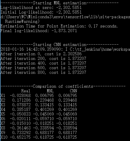
因此,这个实验证实了CNN可以完全实现MNL的参数估计与预测功能,特定的模型设定可以使二者等价。而且我们知道,卷积出来的结果中每个选项的效用,其意义是明确的。
Consequently, this experiment proves that a simple CNN could function exactly as MNL given certain specification. Moreover, each parameter of this CNN is explainable, although in most other CNNs we do not care much about the explanation.
2. 非线性的解释变量:CNN的优势 (Nonlinear Utilities: Advantage of CNN)
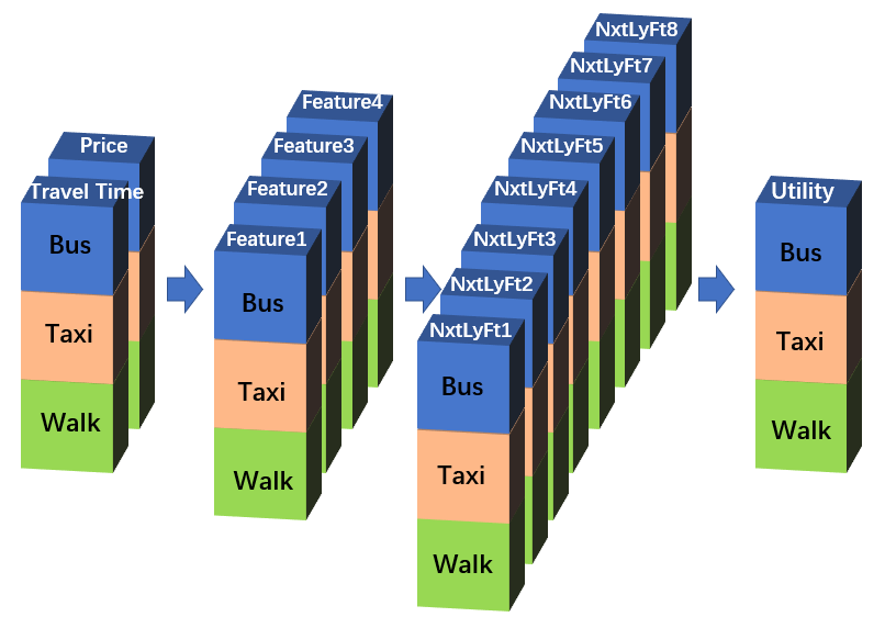
在更进一步之前,不妨做一点小的变换,把上面那张数据结构表侧过来:原来在高度方向上排列的各个备选项不变,把原来在长度方向排列的各个解释变量侧到深度方向,有NVAR个变量就有NVAR个通道,这样就成了下图的形式。此时,每个样本可以看成是尺寸为“NALT * 1”的图片,但有NVAR个通道。
Before go further, let’s take a small transformation to turn the above data-table sideways. All alternatives are still stacked on the hight dimension, however, the explanatory variables, which were stacked on the length dimension before, are now turned to the depth dimension, that means the new picture would have a size of ‘NALT * 1’, and NVAR channels, as shown in the figure below.
这样变换的目的是更直观地利用神经网络的功能。上图中的Utility是经过某一个特定的卷积核[b(TT), b(Pr)]得到的,但在CNN中卷积层中,一般都会在使用多个卷积核,每个卷积核的结果都是一个“NALT * 1”的图片,相当于利用原始变量生成一个新属性,每个备选项在这个新属性上都有一个对应取值。多个卷积核的多个属性结果再在深度方向上叠置,假设有4个卷积核 ,那么就实现了从“Travel Time, Price”到“Feature1, Feature2, Feature3, Feature4”的学习过程。当然,CNN中也常常包括多个卷积层,我们完全可以再把“Feature1, Feature2, Feature3, Feature4”以相同的方式转化为“NextLayerFeature1, NextLayerFeature2,… , NextLaterFeatureN”。在最后一层,我们使用1个卷积核,得到代表每个选项最终得分的“Utiliy”层,然后送入softmax计算概率。形式如下:
Such transformation is to use multiple filters in a layer more intuitively. The ‘Utility’ in the above figure is derived from a certain filter [b(TT), b(Pr)], while a typical CNN would use multiple filters. Each filter will generate a ‘NALT * 1’ output picture, which could be deemed as a new feature coming from the original features. Multiple output-features derived from multiple filters are then similarly stacked on the depth dimension. Supposing we have 4 filters, such calculations are the learning process from the original 2 features ‘Travel Time, Price’ to the new 4 features ‘Feature1, Feature2, Feature3, Feature4’. Moreover, a typical CNN may contains multiple convolutional layers, thus we could similarly generate ‘NextLayerFeature1, NextLayerFeature2, …, NextLayerFeatureN’ from ‘Feature1, Feature2, Feature3, Feature4’. This learning process just goes on, until in the last layer only one filter is used to generate the final score ‘Utility’, which is then sent to the softmax layer.The whole network structure is as follows.
与刚才的等价于MNL的CNN网络相比,这个网络在以下3个方面真正利用了神经网络的优势:1)每个卷积层有多个卷积核;2)有多个卷积层,小小的深度学习;3)每个卷积层要做非线性激活。
Comparing with the simple CNN which is equivalent to MNL, this CNN further employs the advantages of neural networks in 3 aspects: 1) there are multiple filters in each convolutional layer; 2) there are multiple convolutional layers, thus a simple deep learning; 3) each convolutional layer is activated non-linearly.
但与常见的面向图像处理的CNN网络相比,这个网络又有几点不同:1)图片的平面尺寸恒为NALT*1,卷积核的平面尺寸恒为1*1;2)没有池化层;3)不需要考虑padding和stride。归根结底,这个网络只是根据选择问题的数据特点,利用了CNN的形式,因此可能称为“伪CNN”更好一点。
However, this CNN also differs with typical CNNs for computer vision tasks in the following aspects: 1) the size of the sample ‘picture’ keeps ‘NALT * 1’, and the size of the filter keeps ‘1*1’; 2) no pooling layer; 3) no extra padding and stride considerations. Actually, this network just use the extrinsic form of CNN, and might be better described as ‘pseudo CNN’.
下面就来检验伪CNN的能力吧。离散选择模型最大的问题之一就是其效用设定是线性的,而实际情况可能有很复杂的非线性。那么我们来构造一组非线性效用的选择数据。假设我们观察到4个解释变量(X1, X2, X3, X4),它们对选择的影响方式是两两依交互的:V = b1*X1*X2 + b2*X2*X3 + b3*X3*X4 + b4*X4*X1。备选项数设定为4,选择样本数设定为1000。
Now let’s check out the abilities of the ‘pseudo CNN’. One of the greatest problems of traditional discrete choice models is the linear specification of the utilities, which is unreliable in most cases. We could deliberately design a set of choice data with nonlinear utilities: suppose we observe 4 explanatory variables (X1, X2, X3, X4), and they are interacting with each other to constitute the utility, V = b1*X1*X2 + b2*X2*X3 + b3*X3*X4 + b4*X4*X1, the number of alternatives is 4, and the number of choice situations is 1000.
我们拟合3个模型,MNL1是直接使X1~X4的MNL模型;MNL2是使用Feature1=X1*X2, Feature2=X2*X3,Feature3=X3*X4,Feature4=X4*X1这种变换过的新属性的MNL模型,在实际中我们是不可能拟合这个模型的,因为我们并不知道真实的变换关系;模型3是直接使用X1~X4的CNN模型,CNN的网络结构为3个卷积层,卷积核数量分别为20、40、1,前两层采用Relu作为非线性激励函数,最后一层直接线性输出到softmax层。同时,采用70%:30%的比例划分训练与验证集,结果如下。
We estimate 3 models. MNL1 is the MNL model directly using X1~X4 as independent variables; MNL2 is the MNL model using Feature1~Feature4, where Feature1=X1*X2, Feature2=X2*X3,Feature3=X3*X4,Feature4=X4*X1, please notice that this model can not be estimate in practice, since we should have no idea about the real relationship between Feature1~Feature4 and X1~X4; the third one is the CNN model directly using X1~X4, this network contains 3 convolutional layers, each has 20, 40, 1 filters, the first 2 layers have Relu activation and the last layer has no nonlinear activation. The whole data is split into training and test set (70%:30%). The estimating results are as follows.
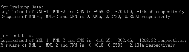
可以看到,MNL1的表现惨不忍睹,由此可见非线性问题的严重性。MNL2模型是“真实模型”,在训练与预测集上的表现差不多,也体现了MNL模型的稳健性。CNN就比较浮夸了,在训练集上的表现好得亮瞎狗眼,而在验证集上的表现则差得亮瞎狗眼,瞎蒙的水平都比它强得多,这显然是极其严重的过拟合。当然,能在训练集上表现那么好,也体现了神经网络的 彪悍之处,只要网络够复杂,什么都不在话下。不过我相信,由于我们的数据实际就是根据MNL2生成的,那么一切比MNL2好的拟合结果都是不可信的。
MNL1 has a quite poor performance, indicating its inability to the nonlinearity. MNL2, the ‘true model’, has similar performance in both training and test data, showing robustness of MNL. In contrast, CNN has a unbelievable wonderful goodness of fit in the training data, and extraordinary poor performance in the test data, which fall far behind randomly guess. Apparently there is a serious over-fitting in CNN. Nevertheless, its great performance in the training data shows the strong power of neural network.
神经网络中有很多对付过拟合的方法,这里就简单地加上L2正则化,重新实验。由于数据都是随机生成的,所以结果与上面完全不一样。
There are many ways to deal with over-fitting in neural network, here we simply add a L2 regularization and re-experiment.
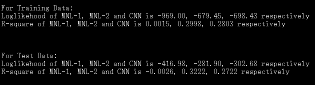
可以看到,这一组数据中,MNL1继续悲催的表现;MNL2表现很好;CNN的过拟合问题已经不大,其在训练集与测试集上的表现均小幅落后于MNL2,但是完全碾压MNL-1。因此可以确信,当解释变量在构成效用时的线性关系不确定时,使用CNN的拟合效果要远远好于MNL。当然,MNL的优势是简单,可解释;CNN一方面是单纯的预测工具,不易解释,一方面要特别小心过拟合的问题。
For the new data, MNL1 / MNL2 keeps very bad / good performance. The over-fitting problem of CNN is basically solved, it falls slightly behind MNL2 in both training and test data , but greatly outperforms MNL1. Consequently, it is safe to say that when the utilities have nonlinear forms, CNN is superior to MNL. On the other hand, MNL has its own advantages in simplicity and interpretability, while CNN is purely a predicting tool and prone to over-fitting.
我还测试了其他一些非线性的效用定义,在代码中给出了其中的3种。无论哪一种,CNN的表现都优于MNL。因此,如果只追求预测的话,以后可以多使用CNN。
I have also tried some other forms of nonlinear utilities, 3 of which are given in the codes. For every nonlinear utility form, CNN outperform MNL.
3. 复杂的选择模型形式:CNN无能为力 (More Complex Choice Model: Inability of CNN)
看到CNN有这样的表现,我进一步期待能否用CNN实现更复杂的离散选择模型,如嵌套Logit模型(nested logit, NL)、混合Logit模型(mixed logit, MXL)。比如说,某个选择问题由于备选项之间的相关关系,实际上应该用NL模型来做的,但我们对此并不清楚,此时还用简单的MNL效果肯定不好,那么用CNN的效果怎么样?我们再通过实验来检验。
Furthermore, I expect if CNN could implement more complicated discrete choice models, such as nested logit (NL), mixed logit (MXL). Supposing we have a choice problem that should be treated using NL because of correlations among alternatives, but we still employ simple MNL and get an unsatisfactory result. Then how about CNN? Let’s try new experiments.
假设NVAR个备选项中,相邻的两个备选项(Alt1与Alt2,Alt3与Alt4,Alt5与Alt6……)是在一个子集中,每个子集有1个自己的参数lambda,表征该子集内的两个选项之间的相关程度。根据这一设定,按嵌套Logit(NL)的规则生成选择数据。在6个备选项,10个解释变量,3000个选择样本的实验中,估计下列3个模型——MNL模型;NL模型;CNN模型,CNN模型的设定同上,并采用了L2正则化,结果如下。
Assuming each two adjacent alternatives (Alt1 & Alt2, Alt3 & Alt4,…) are in the same nest, and each nest has a parameter lambda, representing the degree of correlation among the two alternatives in this nest. 3000 choice situations are randomly generated according to this specification, with 6 alternatives and 10 explanatory variables. 3 models, MNL, NL, and CNN are estimated. The CNN model has the same network structure as before and also use L2 regularization. The results are as follows.
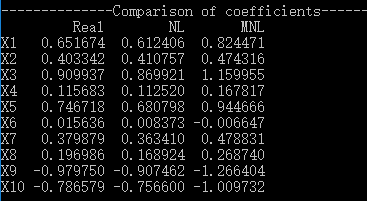
首先,比较一下真实系数、MNL系数、NL系数,可以看到,NL系数与真实系数更接近。当然,不同模型形式的系数不宜直接比较,但显然MNL是存在偏误的。
First, let’s compare the true coefficients and estimated coefficients of MNL and NL. It is clear that NL coefficients are closer to the true settings. Although the parameters of different models should not be compared directly, the MNL results are apparently biased.
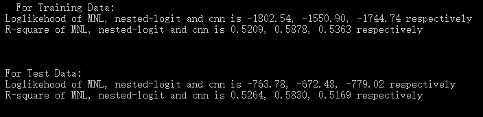
在拟合优度上,3个模型在训练集与测试集上都差别不太大,只有CNN有轻度的过拟合。NL模型作为真实模型,效果当然是最好的。与MNL相比,CNN在训练集上的表现稍好,但是在验证集上的表现略差。这样看来,CNN相较简单的MNL并没有什么优势,它的强大能力无法自动洞察出NL中的嵌套设定。经过许多次实验,该结论一直保持。
As to goodness of fit, NL, the true model, has the best performance unsurprisingly. Compared with MNL, CNN performs slightly better in the training data, while slightly worse in the test data. That is to say, CNN has no advantages over simple MNL, it could no handle the complex tree structure in the NL.
连NL都处理不了,我就没有尝试更加复杂的MXL等模型了。基本可以论断:更复杂、更精细化的离散选择模型形式具有较高的不可替代性,神经网络无法洞察和处理这种微妙的结构,只能靠这些复杂模型本身去解决。
I would not spend time in more complicated MXL model, and just believe that these refined discrete choice models are irreplaceable by CNN.
最后,我想到自己的实际案例数据——五角场万达的消费者空间选择数据中,我也尝试了这样的方法。结果,NL与CNN相比于MNL都有相当明显的改善,NL与CNN的拟合质量相当,还让我产生了CNN可以实现NL的效果的错觉。现在看来,我的数据集既存在效用设定非线性的问题,也存在备选项相关的问题,CNN与NL其实是分别从自己的角度各自解决了一个问题。如果能把CNN与NL的能力再结合起来,那就更理想了。

请问一下,第2节中出现的V = b1*X1*X2 + b2*X2*X3 + b3*X3*X4 + b4*X4*X1,可能会出现这种效用表达式吗?如果有,代表什么含义呢?谢谢
X1, X2, X3, X4的两两相乘只是一种抽象的算例,并没有实际意义。
不过,如果你问的是两个解释变量相乘有没有意义,是有的,代表交互效应或调节效应。一个简单的例子是:X1代表性别(0-男,1-女),X2代表价格,那么b1*X1*X2这一项中的b1就反映了男女在价格敏感度上的差异
有没有可能后面cnn效果不好的原因,就是因为只用了1×1的卷积核。如果把他适当扩大,也许能学到哪些选项之间存在关系。虽然不会像NL那样有显式的预设公式,但是可以学出unobservable的相关性。
补充一下,上面说的相关性是备选项之间的相似性
我可能应该收回上面的问题,不过你最后还是需要得到NALT个Utility,所以从目前看1×1似乎不能避免。