写在前面 Notice
1. 这是一个完全免费的工具。
This is a completely free tool.
2. 我不是专业码农,因此不能保证功能不出现问题。如果你在使用中发现任何bug,请和我联系,除了用户电脑本身的问题以外,绝大多数的问题都可以得到及时解决。
It is hard to get rid of all bugs, and I cannot make guarantee for the functionality of the tool. If you find any bug when using it, please contact with me. I promise that most of the problems (expect those caused only by your computer) could be solved in time.
3. 本工具基于Python 3.6开发,不需要安装运行环境,直接下载、解压后找到exe文件就可以用,坏处是打包后的文件有点大。
This tool is developed based on Python 3.6. Compared with Matlab-based tools, python-based tools do not need additional installation of Runtime and thus could be directly executed by double-clicking .exe file, however, they seems to be much larger in file size.
4. 路径分析的内容很广,本工具目前只是中间版本,希望在以后根据需要不断增加新的功能。
There are so much to do in spatial route analysis. Consequently, this tool is still under developing, and I hope that new methods would be included upon demanding.
下载 Download
方式一:从以下链接下载打包好的exe文件,相对较大,下载并解压缩后,直接运行文件夹中的UtilitiesForSpatialRouteAnalysis.exe文件即可,无需安装python。
Option 1. Download the executable (packed in zip file, named ‘UtilitiesForSpatialRouteAnalysis.exe’) and directly use it without needs to install python.
空间路径分析工具—exe版 (Utilities for Spatial Route Analysis, executable)
方式二:如果有python基础,并安装了python3,那么可以下载下面的zip文件,运行py文件即可。需要注意的是,运行本文件需要一系列的python依赖包,包括:pandas, numpy, tkinter, pickle, sklearn, apyori.
Option 2. Those who have already installed python3 could use following zip file, which contains a py file. Please note that this py file would have to import several modules, including pandas, numpy, tkinter, pickle, sklearn, apyori.
python源代码 (python code for this tool)
功能介绍 Introduction of Functionality
File 文件
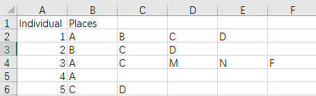
本工具所称的路径,是个体先后到访一系列空间/场所形成的序列。在通过Read CSV Data导入数据时,所需要准备的数据格式是一个csv文件,形式如下。第一列为个体编号或索引,从第二列开始,依次为每位个体的路径。例如,编号为1的个体的路径为“A→B→C→D”,编号为2的个体的路径为“B→C→D”,其中,A/B/C/D/…都是不同的场所。由于不同人的路径长短不一,在读取数据时不会截取特定的长度,而会将第二列以后一切有意义的输入都视为路径,因此,请不要在路径尾部以后增加任何标识符,包括数字、’end’、‘over’之类,它们都会被视为新的场所,留空即可。
In this tool, a route is a sequence of spaces or places an individual has visited successively. When importing route data by ‘Read CSV Data’, users need to prepare a csv file as follows. The first column is the indices of individuals, and the routes start from the second column. For example, the route of individual 1 is ‘A→B→C→D’, and the route of individual 2 is ‘B→C→D’. A/B/C/D/… are the name of different places. Since the routes do not have the same length, we do not cut them to certain length when reading the data, all valid inputs from the second column and afterwards would be recorded to routes. So when a route ends, please leave the following columns empty and do not add anything, including numbers, ‘end’, ‘over’, or any placeholders, they would be mistakenly viewed as new places.
这样的路径数据可以通过多种方式获得,如问卷、GPS、手机大数据等。面向该类数据,本工具集成了一些有趣的分析方法,希望为研究者提供便利,目前主要包括路径聚类、空间关联、路径预测三部分。
Such data could be acquired by questionnaire, GPS, mobile phone big data, etc. This tool provides several interesting methods for this kind of data, including clustering of routes, association among places, and route predicting. Hopefully it will bring convenience for the researchers.
Clustering 聚类
路径聚类的目的是从成百上千的观察路径中找出不同的模式,更进一步,每种模式有自己的原型,从而提取少量的典型路径。由于路径数据是非结构化的,因此传统的聚类算法难以应用。本工具的策略是首先测度路径之间的两两相似度(Analyze Route Similarity),输出结果是一个N*N的相似度矩阵,其中,N为路径的数量。将该矩阵按行求平均,即得到每条路径与所有路径的平均相似度(Mean Similarity with All Routes),平均相似度高的路径当然具有较强的典型性。然而,有的路径虽然能代表一部分路径,但由于与其他路径的相似度均较低,导致其与所有路径的平均相似度被拉低,为了更全面地发现不同模式,提取典型路径,还是需要基于相似度矩阵对路径进行聚类(Affinity Propagation Clustering),得到的结果是一个典型路径表,第一列为个体编号,第二列为典型路径,第三列为该典型路径代表了多少条路径,可以看作是其所对应的类别的大小。
Route clustering is to find several modes from hundreds and thousands of observed routes. Furthermore, we hope that each mode has a representative route, so we could extract typical routes. Since route data is not structured, it is not fit for many traditional clustering algorithms. To solve this problem, we firstly measure the similarity among each pair of routes by running ‘Analyze Route Similarity’, and the output is a N by N similarity matrix, where N is the number of observed routes. We could easily get mean similarity for each route by running ‘Mean Similarity with All Routes’, obviously, the route with larger average similarity would be more typical, However, there might be a route which is able to represent a friction of routes, but has quite low similarity with other routes, as a result, its average similarity with all routes is not as high as expected. Therefore, in order to find different modes, we need to run clustering analysis (‘Affinity Propagation Clustering’) based on similarity matrix. The output is a table of typical routes, the first column is the indices of individuals, the second column is the typical routes, and the third column is the number of routes represented by the typical routes, or saying, the size of the corresponding clusters.
Association 关联
路径将不同的场所串联起来,因此我们可以通过路径数据分析场所之间的关联。最基础的关联是两个场所在同一条路径中共同出现,我们可以执行Co-occurrence Matrix得到M*M的共现矩阵,其中M是场所的数量,矩阵中的元素代表了既到访了场所A、又到访了场所B的个体数量。可以进一步想像一个空间网络,各个场所是网络节点,它们之间的共现次数是网络联系的强度。基于该网络,我们可以运行核心/边缘分析(Core/Periphery: Coreness),通过核心度指标推断各场所在网络中的角色。核心度越高的场所,与其他场所的综合共生性越强,越能在网络中发挥联动效应。如果我们特别关注两个特定场所的关联性,可以运行Probabilities Concerning Two Places,将一个场所(Y)设定为目标场所,另一个场所(X)设定为条件场所,工具将计算一系列概率,如到访X的人中也到访Y的概率,从中可以推断X与Y是否具有潜在的带动关系或竞争关系。最后,本工具还可以执行类似于“啤酒尿布问题”的关联分析(Apriori),根据一些阈值标准,提取形如“如果去了A(或A1, A2, …),就会去B”的关联规则。
Routes connect different places, so we could analyze association among places via route data. The simplest association is co-occurrence of two places in a single route. We could run ‘Co-occurrence Matrix’ to get a M by M matrix, where M is the number of places. The values of this matrix represent the number of individuals who have visited both place A and place B. Going a step further, we could image a space network, whose nodes are places and whose connections are co-occurrence relationship. Based on this network, we could run ‘Core/Periphery: Coreness’ to estimate coreness of each place, which reflects the role of the place in the network. The place with larger coreness is expected to have more coupling effect with other places in the network. If you are pretty interested in the relationship of specific two places, you can run ‘Probabilities Concerning Two Places’. By setting one place (Y) as the target place, and another place (X) as the condition place, this tool would calculate several related probabilities, such as the percentage of people also visit Y among those visit X. From these probabilities, you might find potential stimulating or competing relationship. Finally, this tool provides ‘Apriori’ algorithm, which is used to extract rules like ‘if A (or A1, A2, …), then B’, given certain thresholds.
Prediction 预测
预测部分的基本任务是建立一个模型,能够估计任意一条路径的概率。我们认为输入的数据——不论是大数据还是小数据——只是总体中的一个样本,因此,如果一切概率的计算都完全依赖观察数据的频数和比例,是不够合理的。由观察数据建立背后的模型,再由模型输出概率是更好的替代方案。本工具使用的模型是适合于序列数据的循环神经网络,这种深度学习的方法已经在类似的语言序列中取得很好的效果。由于是深度学习,所以希望用户能够提供尽可能多的路径样本,形成空间路径的“语料库”。在通过Recurrent Neural Network命令建立模型后,可以运行Route Probability去计算任意一条路径的概率,即使这条路径从未在样本中出现过。用户也可以运行Step Probability,计算在已知之前路径的情况下,个体下一步目的地的单步选择概率。最后,基于这些概率,用户可以通过集束搜索方法找到一条最大概率的路径,该路径显然具有较高的典型性。
The essential task of prediction is to set up a model, which should be able to calculate the probability of any route. We believe that the input data, no matter big data or small data, is just a sample from population, consequently, it is not a satisfactory way that all calculation of probabilities are purely relying on the counts and percentages directly derived from observed data. A better choice is to set up a model behind the data and let the model output probabilities. The mode we used is recurrent neural network, a deep learning approach which has proved to be quite successful in a similar area of predicting language probabilities. As a deep learning algorithm, it need as many data as possible. Users could estimate a RNN model by running ‘Recurrent Neural Network’, and then run ‘Route Probability’ to calculate the probability of an arbitrary route, no matter whether it is included in the sample. Users could also run ‘Step Probability’ to calculate the probability of choosing the last place of a route as the next destination, given that the individual has visited previous places of the route. Finally, users could run ‘Beam Search for Typical Route’ to find a route with the largest probability and thus quite typical.
视频示例 Video Demo
下面的视频简要介绍了本工具的各项功能。
The video below briefly introduce the functions of this tool.
下面的视频重点介绍了在本工具的路径聚类功能中,如何通过调整偏好值改变聚类结果。
The video below focus on how different preference settings affect the result of route clustering.
算法 Algorithms
(1) 路径相似度 Route Similarity
采用Levenstein Ratio定义路径相似度,该指标借鉴于自然语言处理中的字符串相似性指标。
Route similarity is measured by Levenstein Ratio, which is often used in NLP for measuring similarity of strings.
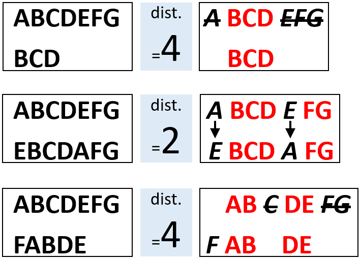
Levenstein距离(或称编辑距离)是将一个字符串转化为另一个字符串所需要的最小编辑次数,包括增加字符、替换字符、删除字符。例如,下图中,从字符串“ABCDEFG”转化为字符串“BCD”,需要删除最开始的“A”和最后面的“EFG”,因此有4个删除操作,两个字符串之间的Levenstein距离为4。这是个非常简单的例子,也有些例子没那么直观,例如:从字符串”ABCDEFG”转化为“FABDE”,需要在头部增加“F”,然后删除中间的“C”和尾部的“FG”,共4个操作(1个增加操作+3个删除操作),Levenstein距离也是4。幸运的是,Levenstein距离的计算有非常简洁高效的算法,不管这种转化是否直观,都很容易实现。可以想像,两个字符串的Levenstein距离越大,它们越不相似。
Levenstein Distance (LD, or Edit Distance) is the minimum operations needed to convert from one string to another. The types of operations include insertion, removal, and substitution. For instance, if we want to convert from ‘ABCDEFG’ to ‘BCD’, we just need to delete ‘A’ and ‘EFG’, the 4 operations of removal define a LD of 4 between two strings. For a more complex example, we want to convert from ‘ABCDEFG’ to ‘FABDE’, we need to add a ‘F’ at the beginning of the string, and then delete ‘C’ in the middle and ‘FG’ at the end. LD is also 4, for 1 insertion and 3 removal. Fortunately, there is an efficient algorithm for LD, which makes the calculation very easy. Obviously, the larger the LD between 2 strings, the less similar they are from each other.
进一步地,Levenstein Ratio被定义为以下公式。注意到该指标除了考虑Levenstein距离之外,还考虑了两个字符串本身的距离,这是非常合理的设定。例如,字符串“AB”与“A”之间的Levenstein距离是1(只需删除最后的”B”),而字符串“ABCDEFGHIJKLMNOPQ”与“ABCDEFGHIJKLMNOP”之间的Levenstein距离也是1(只需删除最后的“Q”),但是后一组的两个字符串要长的多,仅为1的距离就显得微不足道了,因此它们明显比前一组更相似。用Levenstein Ratio进行计算,前一组为0.67,后一组为0.97,这就很合理了。Levenstein Ratio取值在0~1之间,越高则越相似。
Levenstein Ratio (LR) is further defined as follows. Notice that it takes both LD and the length of two strings themselves into consideration, which is quite reasonable. For example, the LD between ‘AB’ and ‘A’ is 1 (one removal operation of ‘B’ at the end), and the LD between ‘ABCDEFGHIJKLMNOPQ’ and ‘ABCDEFGHIJKLMNOP’ is also 1 (one removal operation of ‘Q’ at the end), however, the length of the 2nd group of routes are quite longer, thus a LD of 1 sounds trivial. Therefore, the routes in the 2nd group are more similar with each other than the 1st group. When calculating LR, the 1st group is 0.67, the 2nd group is 0.97, that’s exactly what we expect. LR is ranged between 0 and 1. Higher LR suggests larger similarity.

当我们以一个字符表示一个场所时,则路径可表示为有序的字符串,例如:字符串“ABC”即代表了路径“场所A→场所B→场所C”。因此,用于测度字符串相似性的Levenstein Ratio可以同样地测度路径的相似性。当有N条路径时,它们的两两相似性将构成一个N*N的对称矩阵,即Levenstein Ratio矩阵,或称为相似度矩阵。
When a place is represented as a character, then a route becomes a ordered string. For instance, a string of ‘ABC’ refers to a route of “Place A → Place B → Place C “. Consequently, LR could be generalized to measure the similarity of two routes. For totally N routes, we could get a N*N matrix of pairwise similarities, that is Levenstein Ratio matrix, or saying, similarity matrix.
(2) 路径聚类 Clustering of Routes
本工具采用相似性传播算法(AP)对路径进行聚类。
This tool apply Affinity Propagation (AP) algorithm to run clustering analysis for routes.
AP聚类的优势是直接基于数据之间的相似度,而是原始数据本身,因此对数据结构没有要求。显然,路径数据是典型的非结构化数据,不能直接适用于经典的K-means等算法,而用AP则正合适。另一方面,AP聚类的输出结果是“原型”,每个原型对应一个类别,认为类别中的数据可以被原型所代表。 因此,AP聚类所找到的原型就是典型路径。
The greatest advantage of AP is no assumption upon the data structure, because it is based on similarity among raw data, instead of raw data itself. Apparently, routes are not structured data, thus we can not directly use some classical algorithms, such as K-means, at this time, AP can save us. In addition, the results of AP is a set of so-called ‘exemplars’. Each exemplar corresponds to a cluster, and all cases in that cluster are believed to be represented by that exemplar. In this application, the exemplars found by AP could be viewed as typical routes.
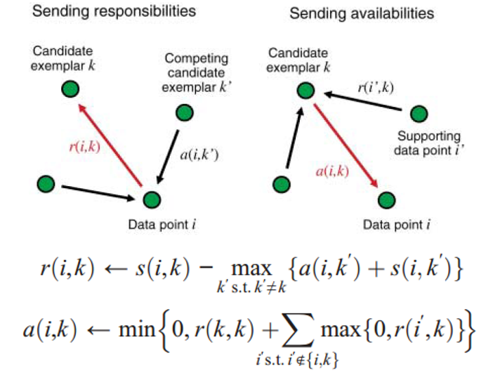
AP聚类的基本原理如上图,反映了各个数据点之间传播相似度的过程。其中,r(i,k)是i向k传播的responsibility,可以理解为i希望自己被k(而不是图中其他竞争性的潜在原型k’)代表的程度,a(i,k)是k向i传播的availability,可以理解为k希望作为原型代表i的信心,这种信心来自图中其他数据点i’的支撑。
The basic principle of AP is as above, which shows the process of affinity propagation among data points. r(i,k) is the responsibility propagated from i to k, it is some kind of degree that i hopes it could be represented by k (instead of other competing candidate exemplar k’); and a(i,k) is the availability propagated from k to i, it is some kind of confidence that k holds from other supporting points i’ to be a exemplar to represent i.
AP聚类的主要参数是各个数据点的偏好值,代表了研究者认为(或希望)该点能够成为原型的程度,偏好值越高的点越有可能成为原型。另一方面,偏好值的大小决定了类别数量,偏好值越大,就好像大家都在抢着当原型一样,会得到相对较多的类别数;反之,偏好值越小,就好像大家都不想当原型,而希望被别的点代表,会得到相对较少的类别数。在默认设置中,所有点的偏好相同,均等于相似度矩阵的中位数。AP聚类会根据偏好值设定自动估计出类别数(即典型路径的数量),但个人感觉,默认设置下这个数量经常会显得过多。Matlab中可以指定类别数,再进行聚类,python中不可以,只能人工改变偏好后反复尝试。如果想设定明确的类别数,可以在本工具中导出相似度矩阵,然后再在Matlab中运行AP聚类。
The key parameter of AP is preference of each data point, which representing the degree that researchers believe (or hope) a data point would be a exemplar. The higher the preference, the more likely that point would be a exemplar. In addition, preferences also influence the number of clusters in an interesting way. When we use larger preferences, it would sound like all points are competing to become exemplars, and we will get relatively more number of cluster; in contrast, if we use smaller preferences, it would sound like each point is trying to escape from being chosen as an exemplar, and we will get relatively small number of cluster. By default, preferences of all points are set to a single value, the median of similarity matrix, so we have no assumption upon which point should be given priority to become a exemplar. AP would derive the number of clusters (i.e. the number of typical routes) based on preferences automatically, however, this number seems to be too large in many cases. We can preset the number of clusters in Matlab, but it is not available in python, and the only way to change the number of clusters is to change preferences manually. As to this problem, we could export the similarity matrix from this tool, and then use Matlab to deal with it.
更多算法的细节请参考以下文献。
For more technical details, refer to the following paper.
(3) 场所在网络中的核心度 Coreness of a place in the network
核心度是社会网络分析中核心/边缘分析的经典指标,为此,我们需要首先建立场所网络。如果某个体既去了场所A,也去了场所B,那么A与B的网络联系加1。通过这种方式构建所有场所之间的“共现矩阵”,其元素代表既去过“行场所”,又去过“列场所”的人数,该矩阵即定义了网络联系。
Coreness is a classical index of core/periphery analysis in social network analysis. In order to use it, we need to build a network of places at first. If an individual goes to both place A and place B, then the association of A and B increase for 1 unit. By this way, we could set a Co-occurrence matrix for all places, the element of which represents the number of individuals who go to both the place of the row and the place of the column. This matrix define the network connections.
核心/边缘分析认为,AB之间的网络联系与A、B各自的核心度成正比,这种思想很像不考虑空间阻抗的重力模型,核心度的角色相当于重力模型中的规模或吸引力,只不过后者是给定的,而核心度正是我们要求解的。根据这一假设,我们可以得到各场所之间的期望联系矩阵,合理的核心度取值将使期望联系矩阵与实际联系矩阵尽可能相似,如下图所示。
In core/periphery analysis, the association of A and B is assumed to be proportional to the coreness of A and B. This idea is quite similar to gravity model without considering spatial impedance. The role of coreness is just like the scale/attractiveness in gravity model. According to this assumption, we could obtain a expected association (co-occurrence) matrix, and we have already got the observed association (co-occurrence) matrix. The most appropriate values of coreness would make these two matrices as similar as possible, as shown below.

具体的求解采用梯度下降法,通过迭代更新核心度值, 逐渐减少期望联系矩阵与实际联系矩阵之间的均方误差。根据惯例,标准化核心度是将核心度标准化至模数为1。
We are using gradient descent algorithm to gradually decrease the mean square error between observed and expected association matrices. According to convention, standardized coreness would have a norm of 1.
算法停止后,会报告期望联系矩阵与实际联系矩阵之间相关系数,如果这个系数比较高,则说明Link(AB) = K * Coreness(A) * Coreness(B)的假设成立。此时,核心度高的场所具有较高的网络乘数效应,因为它与其他所有场所的联系都会乘以一个较高的值。
After the gradient descent algorithm converges, the correlation coefficient between observed and expected association matrices would be reported. A large correlation coefficient suggests that the assumption of ‘Link(AB) = K * Coreness(A) * Coreness(B)’ is reasonable. The higher the coreness of a place, the more important it would be in the place network, because the association of any place with it would be multiplied with a large value.
在求得所有N个场所的核心度以后,算法会推荐核心度最高的K个场作,作为核心场所,其原理如下。设核心场所的数量为n,然后构建一个理论上的二值核心度向量——核心度最高的n个场所取值为1,其余场所取值为0,计算这个理论上的二值核心度向量与实际求得的核心度向量的相关系数。将n从0(没有核心场所)变到N(全都是核心场所),上述相关系数将先上升(核心场所太少),后下降(核心场所太多),其取最高值时的n就是我们要找的K。
After we get the coreness of all N places, the algorithm would recommend K places with the largest coreness as core places. The way of recommendation is as follows. Assuming the number of core places is n, we could set a new theoretically binary coreness vector, which has values of 1 for the n places with the largest coreness, and 0 otherwise. The correlation coefficient of this vector and the real-value coreness vector could be calculated. Changing n from 0 (no core places) to N (all places are core places), this correlation coefficient would rise at first (too few core places), and then drop down (too many core places). When it reaches the peak value, we get our K.
关于核心度(以及核心/边缘分析)的进一步的技术细节,可以参阅以下论文。个人认为,当网络是多值而非0/1二值时,核心度比中心度更有意义。
As to more details of coreness (and core/periphery analysis), please refer to the paper below. Personally, I believe that coreness is better than centrality for real-value (instead of 0/1) network.
S. P. & Everett M. G. Modiels of core/periphery structures[J]. Social Networks, 1999, (21): 375-395.
(4) Apriori
Apriori是经典的关联规则算法,在国内常用于解决著名的啤酒尿布问题——虽然据说这是一个伪命题。Apriori的主要任务是从数据中提取形如“A→B”(或:“如果A,则B”)的关联规则,在本应用可解释为“去过A,则很可能也去B”,其中A可以是多个场所的集合(A1, A2,…),而B只能是单个场所。这种规则实际上一符合一定标准的频繁项集,而最常见的标准是两个——置信度(Confidence)与支持度(Support)。
Apriori is a classical association rule algorithm, which is often mentioned in solving the so-called problem of beer and diaper. Apriori is to extract association rules like ‘A→B’ (or, ‘if A, then B’), in the context of this application, such rules could be explained as “if someone visits place A, he tends to also visit place B”. A could be a set of multiple places (A1, A2, …), while B must be a single place. These rules are actually frequent item-sets that meet certain criteria. The 2 most frequently used criteria are Support and Confidence.
对于“A→B”的规则而言,置信度就是去过A的个体中,也去过B的比率,即条件概率P(B|A);支持度则是同时去过A和B的个体占总样本的比率,即联合概率P(AB)。例如,100个人中,如果有20个人去过场所A,这20人中,又有10个人去过场所B,则“A→B”的置信度P(B|A)=10/20=0.5,支持度P(AB)=10/100=0.1。置信度和支持度都应该有一个下限阈值。支持度过低时,置信度高只是偶然造成的,例如只有1个人去过A,正巧那个人也去了B,则“A→B”的置信度是100%,却没有意义;置信度过低时,支持度虽高,但指向性不明确,例如有很多人同时去过A和B,但也很多人只去了A、没有去B,则“A→B”同样不成立。
The confidence of a rule ‘A→B’ is the conditional probability of people visiting place B given that they visit place A, or saying P(B|A); and the support is the joint probability of people visiting both A and B, or saying P(AB). For instance, if 20 of 100 individuals have visited placed place A, and 10 of them have also visited place B, then the confidence of the rule “A→B” is P(B|A)=10/20=0.5, the support is P(AB)=10/100=0.1. We should set the thresholds for both confidence and support. When the support of a rule is too low, even the confidence is high enough, it might be just attribute to chance; on the other hand, when the confidence of a rule is too low, we can not judge the direction of the rule.
另一个更高级的标准是提升度(Lift)。如前所述,“A→B”要想成为关联规则,就要满足一定的置信度要求,去过A的人去B的概率P(B|A)较高。但是,如果我们即使不考虑“去过A”这一条件,仅观察去没有过B,就发现P(B)已经足够高了,那么“去过A”这一条件对“会去B”就没那么大的意义了。例如,有三条路径:“A→B→C”、“A→C”,“B→C”,由于有2个人去了B,所以P(B)=2/3=0.67,而在去过A的2个人中,只有1个人也去了B,所以P(B|A)=1/2=0.5,还不如P(B)高,那么在这种情况下,如果我们要推荐B,就没有必要瞄准已经去过A的人,认为他们更有可能去B了,因为效果还不如随机推荐,因此,即使我们把置信度下限设为0.5,“A→B”也不值得成为一条规则,因为相比于不知道A的先验概率P(B),知道A信息以后的后验概率P(B|A)没有带来提升。关联规则“A→B”的提升度即是P(B|A) / P(B),我们一般希望其至少大于1。
Another advanced criteria is Lift. As mentioned before, ‘A→B’ should have a high enough confidence P(B|A) to become a rule. However, if we observe a high P(B) without knowing whether or not individuals visit A, then ‘visiting A’ would be not important for ‘visiting B’. For instance, there are three routes “A→B→C”、“A→C”,“B→C”, then P(B)=2/3=0.67, and P(B|A)=1/2=0.5, which is even less than P(B). At this time, if we want to recommend B to a person, it is not necessary to aim at those who visit A and expect they are more likely to visit B, since it would be even better to recommend B to a random person. Consequently, even though we lower the threshold of confidence to 0.5, ‘A→B’ should not be a rule, because there is not lift for the probability of visiting B given the information of visiting A. The lift of a rule ‘A→B’ is defined as P(B|A) / P(B), and generally we hope it should larger than 1 for a satisfactory rule.
关于Apriori算法的进一步技术细节可参阅以下论文。
For more technical details of Apriori , please refer to the following paper.
(5) 利用循环神经网络预测路径 Predicting routes using recurrent neural network
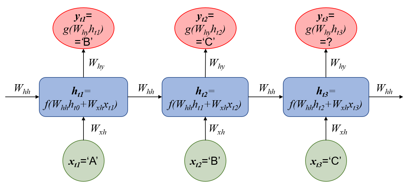
循环神经网络(RNN)主要用于预测序列数据,因此适合于预测路径。在每一时刻,RNN单元的输入(x)是个体当前所在的场所,而输出的预测结果(y)是下一步要去的场所,输入到输出是以隐藏层(h)为媒介的,而隐藏层是沿着时间序列前后连接的,换句话说:当前时刻隐藏层的输出结果(ht)不仅取决于当前的输入(xt),也取决于上一时刻隐藏层的输出(ht-1)。例如,“…→A→B→C→…”是一条路径的片段,个体到访A、B、C的时间点分别为t1, t2, t3,则RNN的结构如下图。式中,wxh,why, whh分别是连接输入层与隐藏层,隐藏层与输出层,上一时刻隐藏层与本时刻隐藏层的权值,f与g为非线性激励函数。
Recurrent neural network (RNN) is mainly used for predicting sequence data, so it is suitable for predicting routes. Each time, the RNN unit takes the input of the current place of an individual, and outputs his/her choice for the next place. There is a hidden layer connecting the input and output layers, and hidden layers are connected to themselves across time. In another word, the output of the hidden layer at time t (ht) depends not only on the current input (xt), but also the output of the hidden layer at the previous time (ht-1). For example, “…→A→B→C→…” is a piece of a route, and the times for visiting A, B, and C are t1, t2, t3 respectively, then the network structure of RNN is as follows, where wxh,why, whh are weights connecting input and hidden layers, weights connecting hidden and output layers, and weights connecting previous and current hidden layers, f and g are nonlinear activation functions.
在输入中没有考虑描述下一步备选场所的物质环境特征(比如距离、面积等),而只是使用当前场所的虚拟变量(即one-hot编码),其实质是使用之前的路径序列预测下一个路径点,这种工作机制类似于语言模型(在一句话中用前面的词预测下一个词)。因此,这种方法并不能用于预测物质环境改变后的路径,而只是用于更深入地理解现状路径。当然,也可以把这些变量纳入神经网络,只是由于不同的应用场景下考虑的变量不一样,不容易做成通用的工具。
The input of this RNN do not consider the features describing the physical environment (such as distance, areas, etc.) of alternative places for the next step, and only use the dummy variable (or saying, one hot encodes) of the current place. So this RNN is actually predicting the next place just according to preview places. which is similar to language model. As the result, it can not predict routes when physical environment changes, and is just for deepening our understanding of current routes. It is certainly possible to introduce these features into neural networks, but we did not make it a general tool for the difficulty of setting different features in different applications.
(6) 集束搜索与最大概率路径 Beam search for the largest probability route
在建立一个RNN以后,可以不断预测下一步的场所,从而得到一条路径。我们可以设想找到一条概率最大的路径,它应当非常具有典型性,那么,如何根据RNN每一步输出的选择概率选出一个场所,使最后生成的路径概率最大呢?
A RNN allows us to calculate the probability of a route and generate a route by continuously predicting the next destination. We would like to find a route with the largest probability, and view it as a typical route. Now the problem is how to choose a destination according to the probability distribution outputted by RNN at each step, so that the final route would has the largest probability?
最简单的逻辑是每一步都找概率最大的场所,这种方法被称为贪婪搜索,然而在许多情况下,贪婪搜索都会错过最大概率路径,因为该路径并不一定在每一步的场所选择概率上都是最大的。集束搜索很好地解决了这一问题,它在每一步预测时都保留K条当前概率最高的路径(注意:是当前路径的概率,而不是当前那一步选择目的地的概率),以用于下一步的搜索。
The most straightforward logic is to choose the place with the largest probability at each step, and this way is called Greedy Search. However, in many cases greedy search would miss the largest probability route, because there might be a place whose probability is not the largest, but having better successors. Beam Search could well solve this problem, it keeps K routes with the largest probabilities at each step (note: probabilities for the current routes, not for the destinations at that single step) for searching at the next step.
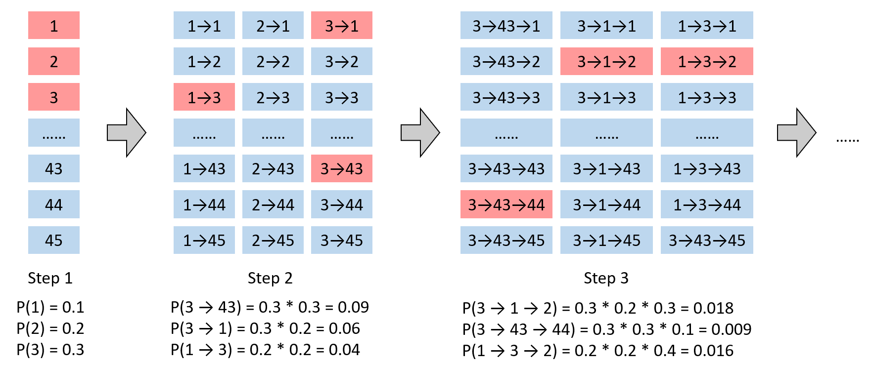
例如,下图中有45个场所,我们取K=3。第一步时,概率最高的3个场选是1, 2, 3。如果第一步选择了1,那么下一步计算1→1, 1→2, 直至1→45的概率;如果选择了2,则下一步计算2→1, 2→2, 直至2→45的概率;同样地,我们也要计算3→1, 3→2, 直至3→45的概率,这样就有3*45=135个概率,我们从中再选出概率最高的3条路径,分别是3→43, 3→1, 1→3。进入第三步,如果前两步选择了3→43,那么依次计算3→43→1, 3→43→2, 直至3→43→45的概率;如果前两步选择了3→1,那么依次计算3→1→1, 3→1→2, 直至3→1→45的概率;类似地,我们也计算1→3→1, 1→3→2, 直至1→3→45的概率,这样又有了3*45=135个概率,我们再从中选出概率最高的3条路径,此时,注意到概率最高的路径已经是3→1→2了,如果我们采用贪婪搜索,第二步选中了43,那么就会错过这条路径。这样的过程依次类推。
For example, there are totally 45 places as alternatives, as shown in the following figure, and we set K=3. At the first step, the 3 places with the largest probabilities are 1, 2, 3. Assuming we choose place 1 at the first step, so we have to calculate the probabilities of routes ‘1→1’, ‘1→2, ‘…, ‘1→45’; assuming we choose place 2 at the first step, so we will also calculate the probabilities of routes ‘2→1’, ‘2→2’, …, ‘2→45’; similarly,, we would also calculate the probabilities of routes ‘3→1’, ‘3→2’,…, ‘3→45’. As the result, there would be totally 3*45 = 135 routes, from which we would choose 3 routes with the largest probabilities, ‘3→43’, ‘3→1’, ‘1→3’. Now let’s move to the third step. Assuming we have chosen ‘3→43’ at the first 2 steps, we will calculate the probabilities of routes ‘3→43→1’, ‘3→43→2’, …, ‘3→43→45’; assuming we have chosen ‘3→1’ at the first 2 steps, we would calculate the probabilities of routes ‘3→1→1’, ‘3→1→2′,…’3→1→45’; similarly, we would also calculate the probabilities of routes ‘1→3→1’, ‘1→3→2’,…, ‘1→3→45’. Again, there would be totally 3*45=135 routes, from which we would choose 3 routes with the largest probabilities. At this time, the route with the largest probability is already ‘3→1→2’, not ‘3→43→#’. If we apply greedy search, we would choose place 43 at the second step, and thus miss this route.
K是集束搜索的唯一参数。K越大,集束搜索得到的路径真的是概率最大路径的信心越强,但相应的计算成本也更高,反之亦然。当K=1时,集束搜索退化为贪婪搜索。
K is the only parameter of beam search. A larger K would give more confidence that the route outputted by beam search would really has the largest probability, however, it would more computational expensive, vice versa. When K=1, beam search is just the same as greedy search.
